
Category: Carbon Footprints

  • The air onlylooks the same.

    The air onlylooks the same.

    ATLASInsights / Atmosphere

    The Keeling Curve · A short read, a longer view

    Unlock your phone. Make coffee. Take a breath. That last part feels just like it did a lifetime ago. The air has changed.
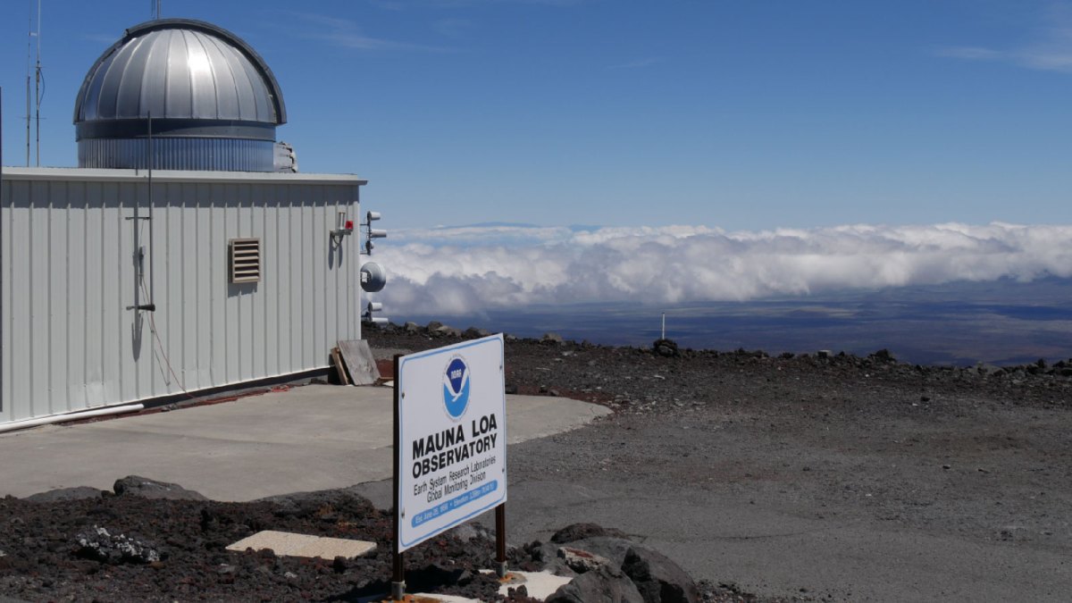
    Mauna Loa Observatory building and NOAA sign on volcanic ground above the clouds in Hawaii.
    Mauna Loa Observatory, Hawaii. Image credit: NOAA / Public Domain

    When Charles David Keeling began measuring CO₂ at Mauna Loa in 1958, the air contained about 315 parts per million. The annual average in 2025 was 427.35 — roughly 427 CO₂ molecules in every million molecules of dry air. Scripps · NOAA

    The Keeling Curve tracks that rise. Watch one lifetime unfold. Then pull back a thousand years. Then eight hundred thousand.

    One lifetime. More CO₂.

    Monthly CO₂ at Mauna Loa · 1958–2025.

    427.49ppm · December 2025
    One lifetime. More CO₂.CO₂ · ppm3003403804201958198020002025
    The teeth follow the seasons. The long climb is mainly driven by fossil-fuel burning.

    NOAA GML / Scripps · dry-air CO₂ concentration

    Chart by PROJECT ATLASNOAA · NASA · Scripps · 2 Degrees Institute

    A familiar breath. An unfamiliar story.New to the Keeling Curve? If this changed how you see the air, share the chart on your own website.

    Why the teeth?

    Earth’s two halves have opposite seasons. But they do not cancel each other out: most land lies north of the equator, and northern vegetation dominates the seasonal rhythm. During northern summer, growing plants draw CO₂ out of the air. In autumn and winter, photosynthesis weakens while respiration and decay keep returning it. NOAA: the seasonal cycle

    Opposite seasons. One atmosphere.

    Watch four measured years of CO₂, with a schematic seasonal overlay.

    January 2021
    North · WinterSouth · Summer
    Equal Earth: opposite seasons, one atmosphereEquator · 0°
    SummerWinter

    Equal Earth preserves relative areas. Seasonal colours are schematic, not measured vegetation or carbon flux.

    Four years of seasonal teethMauna Loa CO₂ · ppm · monthly means4104204302021202220232024

    Northern summer draws CO₂ down; northern autumn and winter usually bring it back up as growth slows and respiration and decay continue.

    NOAA GML / Scripps · monthly means, 2021–2024 · map: supplied Equal Earth SVG / Natural Earth

    The seasonal dip does not undo the long climb, driven mainly by burning fossil fuels. Nature’s annual rhythm sits on a rising baseline. The history of the curve

    A longer view changes the picture.

    Ancient air trapped in Antarctic ice puts the displayed pre-industrial CO₂ range at roughly 170–300 ppm over about 800,000 years. The 2025 value stands above it. In that deep-time view, temperature means Antarctica; the modern comparison uses the global average. Ice-core data

    Why care? CO₂ slows heat escaping to space. More of it strengthens warming, even as other influences make temperatures fluctuate. NASA

    Between two cups of coffee, you won’t notice the change. Across one lifetime, it becomes an entire rising line.

    What the charts show

    One lifetime: NOAA’s combined monthly Mauna Loa series, March 1958–December 2025. Early values are from Scripps. These are processed monthly means, not individual readings; the source interpolates missing months. The volcanic interruption from December 2022 to early July 2023 uses Maunakea observations.

    Temperature: annual Mauna Loa CO₂ and NASA GISTEMP v4 global land–ocean temperature, 1959–2025. Temperature is the anomaly relative to 1951–1980, not absolute temperature or a pre-industrial baseline. The 2025 anomaly is +1.19 °C on that basis. Mauna Loa is one CO₂ monitoring site, not a global CO₂ mean.

    The last 1,000 years: the supplied 2 Degrees Institute / Climate Levels CSV, dated 18 September 2026, contains 6,494 values from 1010 to 15 September 2026. It combines an early ice-core-based history with much finer modern atmospheric data. We retain its values and dates; they do not all represent measurements of the same frequency or precision. The export does not supply per-row uncertainty or processing history. The c. 1760 guide marks the conventional start of Britain’s Industrial Revolution, not an instantaneous change in CO₂. Science Museum: industrial context · CO2.earth source page · Climate Levels / 2 Degrees Institute

    800,000 years: CO₂ from Bereiter et al. (2015), stopping at 1850; Antarctic Dome C temperature from Jouzel et al. (2007), relative to the source’s mean of the last 1,000 years. Ages are years before 1950. The two records have different chronologies, sampling intervals and uncertainties. Vertical guides mark selected cold minima, rounded to the nearest thousand years, rather than formal global glacial boundaries. The 2025 Mauna Loa annual mean is a separate CO₂ point; its dashed connector is only a visual guide. We do not append modern global temperature to Antarctic paleotemperature.

    The seasonal map: a conceptual colour layer on the supplied world SVG, synchronized with actual monthly CO₂ for 2021–2024. Yellow means summer and blue winter; intermediate colours show transitions. Seasons are opposite across the equator, but tropical and regional growing cycles differ. The Equal Earth projection preserves relative areas; colours are not measured temperature, vegetation cover or carbon flux. Northern CO₂ usually peaks around May and bottoms out around early autumn. NOAA: seasonal exchange

    Animations reveal existing data. The moving cursor is visually interpolated between samples; numerical readouts use source values. Similar-looking curves alone do not establish causation or precise time lags. Orbital changes and climate–carbon feedbacks both matter in glacial cycles. NASA: the carbon cycle

    Data retrieved 18 September 2026. The lifetime and temperature views end in the last complete year, 2025; the supplied millennium export extends into 2026. Scales stay fixed within each view. In the lifetime and 800,000-year animations, the number and its sample date update once per second for readability; pause or scrub for the source precision. The line continues moving between these readouts. Reduced-motion preferences show a static view with manual scrubbing.
    Source data and references

    NOAA/Scripps monthly CO₂ · NOAA annual CO₂ · NASA GISTEMP v4 · Lenssen et al. (2024)

    Bereiter et al. (2015) · Antarctic CO₂ data · Jouzel et al. (2007) · Dome C temperature data

    CO2.earth ice-core guide · 2 Degrees Institute / Climate Levels · ATLAS Equal Earth world map

    PROJECT ATLAS · Four perspectives on the air we share

    Embed this chart

    The original chart is in English.

  • How Much CO₂ Has Your Car Produced Since It Was Built?

    How Much CO₂ Has Your Car Produced Since It Was Built?

    Follow a car through production, years of driving and the decisions that shape its carbon history.

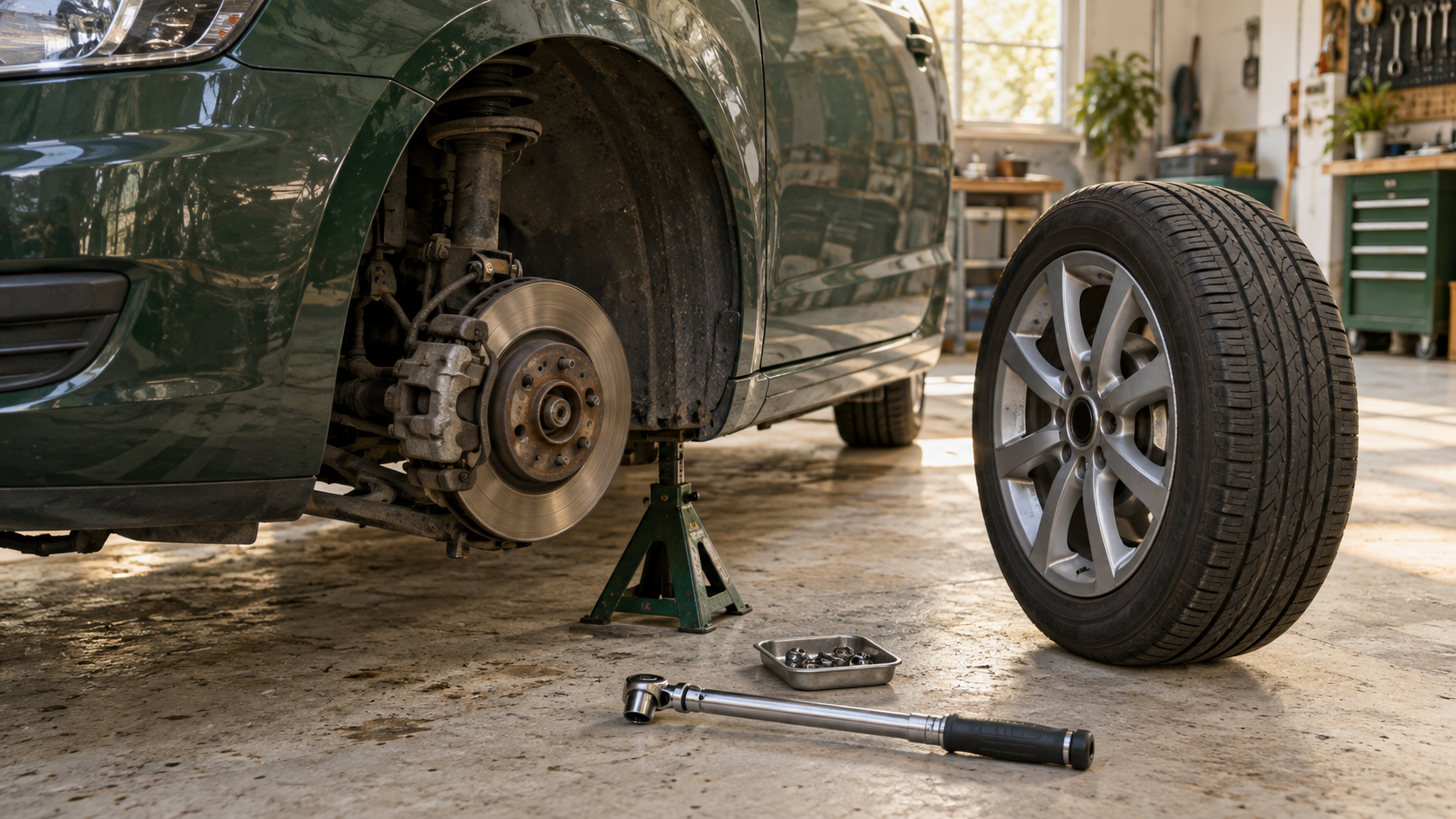
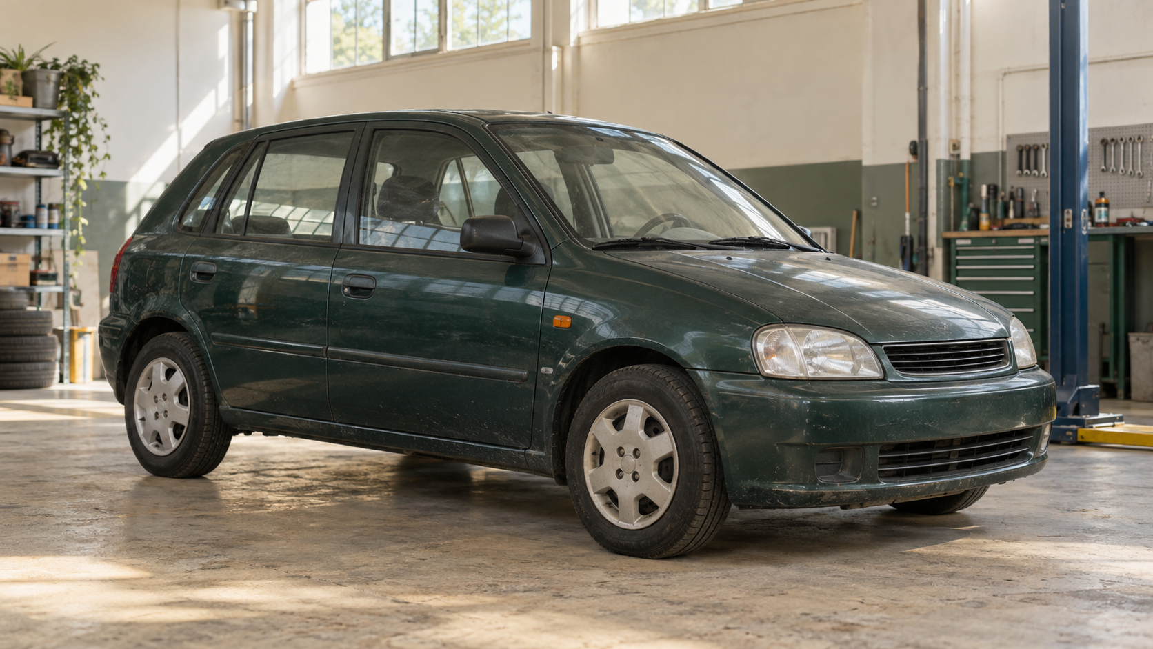
    An ordinary car in a workshop, connecting everyday journeys with the work behind them.
    Illustrative scene.

    A car’s odometer keeps a record of journeys long after their details have faded. It also holds the raw material for a different kind of history: the CO₂ connected to making, fuelling and maintaining the vehicle.

    Consider an illustrative petrol car with 220,000 km on the clock and an average consumption of 10.4 L/100 km. Its fuel use alone comes to 22,880 litres. At 2.34 kg CO₂ per litre of petrol, that is about 53.5 tonnes of CO₂ from combustion.

    Fuel is only part of that history. The car already carried a production footprint before its first kilometre, and servicing adds further events over time.

    So how much CO₂ has your car produced?

    Open the calculator in a full page ↗

    The tonnes behind the kilometres

    The number may feel unexpectedly large because we usually encounter fuel in small purchases, not as a lifetime total.

    For a combustion car, the central calculation is straightforward:

    Distance × average fuel consumption ÷ 100 × CO₂ per litre.

    In the example above, 220,000 × 10.4 ÷ 100 gives 22,880 litres. Multiplying by 2.34 kg CO₂ per litre gives roughly 53.5 tonnes.

    How can the gas weigh so much? Burning fuel joins its carbon with oxygen from the air. The resulting CO₂ therefore weighs more than the fuel itself.

    That is also why one generic “car emission” figure is a poor substitute for your own history. Distance and consumption matter.

    If you have reliable long-run fuel records, use them. Otherwise, the catalogue value is a transparent starting point.

    Time turns a rate into a history

    At an unchanged fuel consumption, twice the distance means twice the fuel-combustion CO₂.

    A conversion gives the history a change of direction. If a petrol car switched to LPG, its fuel use and emissions need to be calculated separately before and after the conversion.

    For LPG, the calculator starts with 20% more litres than the petrol reading: 8.0 L/100 km petrol becomes 9.6 L/100 km LPG. It then applies the LPG factor for the relevant period.

    A carbon history begins before the first kilometre

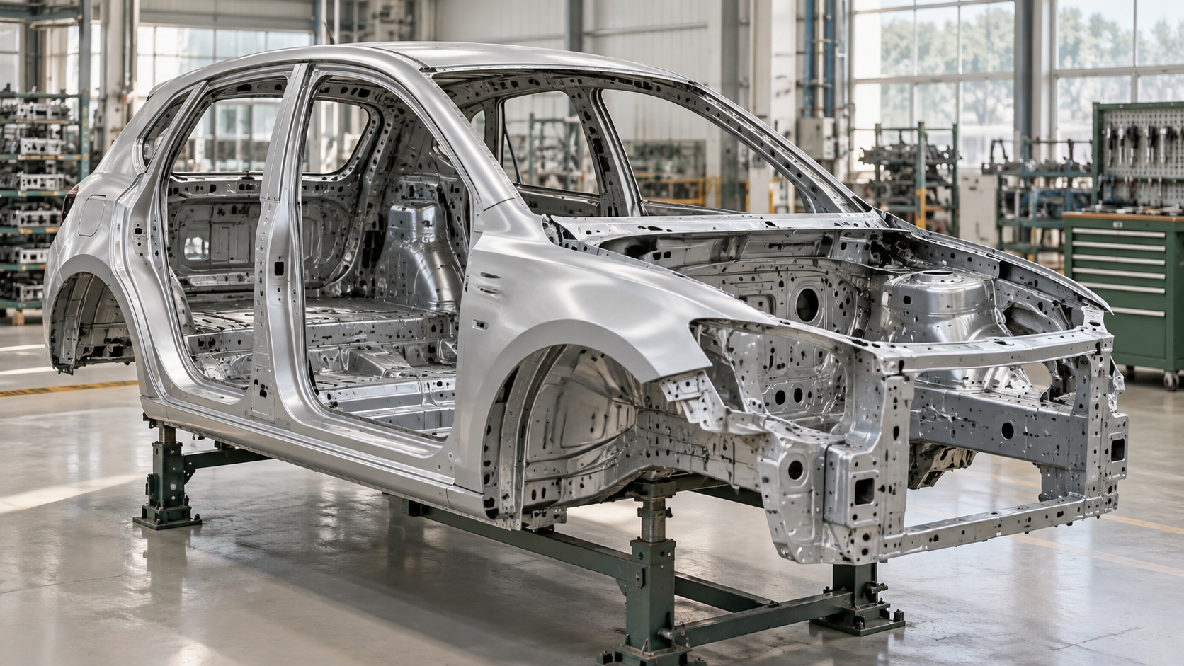
    A vehicle body during manufacture, before it has travelled its first kilometre.
    Illustrative scene.

    At zero kilometres, no driving fuel has been counted. Yet the car has already been made.

    Materials had to be produced and formed, components manufactured, and the vehicle assembled and transported.

    The difficulty is attaching an honest number to those earlier stages. Weight, material mix, manufacturing energy and supply chains all vary.

    The production estimate uses vehicle mass where available, historical material and energy profiles, and a transparent physical-CO₂ inventory.

    The physical-CO₂ inventory draws on historical European material and energy profiles. It is not a claim about a particular factory or supply chain.

    One production event, several owners

    The calculator provides two views. Vehicle history counts production once, at the beginning. Ownership history allocates a share of production to the years you owned the car.

    ATLAS uses a chosen ten-year allocation: 25.6%, 19.3%, 14.6%, 11.1%, 8.5%, 6.5%, 4.9%, 3.7%, 2.8% and 2.1%.

    If you bought a 1994 car in 2018, no production share falls within your ownership period. The vehicle still has a production footprint; it simply sits before your years of ownership.

    Your mileage is also separate from its odometer. Buying at 100,000 km and driving 20,000 km means your ownership history covers those 20,000 km, not the earlier 100,000 km.

    Why the average changes as you drive

    For an illustrative production footprint of six tonnes of CO₂, the production average is 60 g/km at 100,000 km, 30 g/km at 200,000 km and 15 g/km at 400,000 km.

    The million-kilometre explorer counts full production once and adds driving and service events as distance grows. It is a way to see how a fixed beginning is spread across a longer history.

    Servicing leaves steps in the history

    Tyres and brake components being serviced in a workshop.
    Illustrative scene.

    The annual bars show individual replacement events. Tyres, oil, brake parts, shocks, batteries and other components appear when their assumed service interval is reached.

    These are generic schedules and assumed part quantities, not a reconstruction of a particular vehicle’s workshop record.

    The events make timing visible, but extra detail does not guarantee extra accuracy. The calculator keeps the assumptions visible so you can judge their relevance.

    Different fuels change the route to CO₂

    Petrol, diesel, hybrid and electric cars all connect distance with energy, but the route differs. The calculator keeps those routes separate rather than forcing them into one generic number.

  • How Much CO₂ Have I Produced in My Lifetime?

    How Much CO₂ Have I Produced in My Lifetime?

    Your footprint has a history. Explore how the places you have lived and the choices you have made add up—and what a monthly contribution could fund.

    ATLAS / Carbon & everyday life

    Think of the homes you have lived in. The room you grew up in, the first place you rented, the home you return to now. Add the journeys, meals and purchases along the way. What might they amount to over a lifetime?

    You do not need every old energy bill to explore that question. Start with what you remember, then see which changes move the result. The calculator combines published CO₂ factors with simple assumptions to give an approximate range.

    It is an invitation to investigate, not a measurement of your actual emissions. Countries, individual habits and earlier decades can differ substantially from the reference data. The method below explains the shortcuts.

    Start with the life you actually lived

    Your current routine may look little like your childhood. You might have moved countries, changed homes, started driving or changed your diet.

    Begin with one chapter using averages across the whole period. If you want more detail, split it at a move or a change in habits. Enter your own travel as a passenger as well as a driver. Childhood travel can include family journeys; it should not automatically copy the kilometres you drive today.

    The tool applies the same annual profile within each chapter. It does not automatically adjust food portions for age or reconstruct historical electricity systems. Splitting chapters makes your inputs more descriptive, but it does not turn the estimate into a personal emissions record.

    What belongs in your footprint?

    There is more to it than exhaust pipes and heating. The things you buy and the services you use also have supply chains. Consumption accounting follows those connections. Defra’s footprint explanation.

    This calculator adds eight categories: home energy, food, car travel, buses, trains, flights, other goods and services, and public services and infrastructure.

    The last category addresses a useful question: what about a road you use but did not build? Economy-wide footprint accounts can include public consumption and investment. OECD’s accounting framework.

    Here, indirect consumption starts with editable allowances of 1.2 tonnes of CO₂ per person per year for other goods and services, and 0.5 tonnes for public services and infrastructure. These are scenario assumptions, identical across countries—not measured national averages. The private allowance is intended to cover residual supply chains and purchases outside the itemised categories. It does not establish a complete lifecycle total.

    Both allowances count once. Neither is divided again by household size or car occupancy. Try changing them to see how much of your result depends on what happens beyond your direct energy use.

    This calculator counts CO₂ only

    The focus is carbon dioxide, the gas ATLAS aims to remove. Methane, nitrous oxide and aviation’s non-CO₂ effects are excluded. This means the result is not your entire climate footprint. EPA’s explanation of different greenhouse gases.

    Food estimates use the CO₂ component of a UK study of adult diet groups. Applying those groups to other countries, childhood or earlier decades is a shortcut. Diet study, Table 2.

    Travel and fuel calculations use the CO₂-only entries in the UK government’s 2026 conversion factors. Those operating factors are useful reference points, rather than universal lifetime averages. The flight calculation excludes the non-CO₂ warming multiplier. Wood heating includes released biogenic CO₂ without assuming that regrowth immediately cancels it. DESNZ factors and methodology.

    Share the journey, share the car emissions

    Enter the distance you personally travel by car. The calculator multiplies it by the vehicle factor and divides by average occupancy, including the driver. You do not need to divide your kilometres first.

    Using the reference petrol-car factor, 6,000 km produces approximately 0.97 tonnes of operating CO₂ per vehicle. Your allocated share is about 0.64 tonnes with 1.5 occupants, or 0.48 tonnes with two.

    When occupancy varies, the split matters. If you travel 3,000 km alone and 3,000 km with two people, your share is 3,000 + 1,500 vehicle-km. For the combined 6,000 km, enter an effective occupancy of about 1.33.

    Bus and train figures are already allocated per passenger. The tool uses UK public-transport averages as simple proxies, and does not divide them again by car occupancy.

    Flights use economy-class reference trips: about 3,000 km in total for a short return trip and 12,000 km for a long return trip. Adjust the trip count for substantially different distances. These are broad categories, not an airport-by-airport calculation.

    What could €30 a month actually fund?

    The budget has two jobs. First, it funds credits corresponding to ongoing CO₂ emissions. Any money left funds historical removal. Both prices start at an all-inclusive €50 per tonne, with the purchased quantities recorded at the end of each payment month.

    Imagine a historical benchmark of 200 tonnes, continuing emissions of 4 tonnes a year and a €30 monthly budget. The annual €360 contribution allocates €200 to current emissions. The remaining €160 funds 3.2 tonnes of historical removal per year. At that constant rate, reaching the historical benchmark takes 750 monthly payments, or 62.5 years.

    A bigger contribution changes that timeline. So does reducing future emissions: less of the same payment goes towards the present, leaving more for the past.

    At the default prices, €50 funds one tonne in total, split between those two purposes. If current emissions use the entire budget, nothing remains for historical removal. The calculator can therefore return “not reached by age 100”.

    These are funding scenarios, not a guarantee of a finishing age or a claim that project delivery has been verified.

    Read the two curves carefully

    The terracotta curve accumulates estimated emissions through your past and into your future. Changing future habits changes its slope without rewriting your history.

    The green dashed curve adds current-emission credits and historical removal quantities. The readout keeps the two separate. Annual points sum the monthly allocations.

    A crossing means the accounting totals meet in that scenario. It does not establish climate neutrality: avoiding emissions and withdrawing CO₂ from the atmosphere are different interventions. Oxford’s offsetting principles.

    The shaded range combines lower and higher assumptions by category. Published food-study bounds and observed household-energy variation help inform it; the travel and indirect-consumption ranges are exploratory choices. It is not a statistical confidence interval, and your real footprint could lie outside it.

    Where a forest could fit

    ATLAS is exploring new carbon sinks through newly planted and actively managed forests. The question is how a contribution could support traceable removal over time.

    A credible answer needs evidence about the project, its baseline, emissions and carbon storage. A payment or planting record alone cannot establish delivered removal. No tree yield or land entitlement is built into this calculator.

    For now, explore what moves your estimate. Does sharing car journeys make a noticeable difference? What happens if future emissions fall? How much more of your contribution can then go towards the past?

    A short note on the method

    The reference home is anchored to England and Wales household-energy data for 2024. Floor-area scaling and heating efficiencies simplify the calculation. Country electricity factors remain broad proxies; the 15-country menu is organised by HDI, which does not determine emissions. Home-energy data, UNDP country data.

    History ends at the start of 2026. Future funding runs monthly up to age 100, and any selected annual emissions decline compounds once per model year. The page keeps your inputs on your device. Open the calculator’s method panel for sources, coefficients and the remaining assumptions.

  • How Much CO₂ Do My Everyday Actions Emit?

    How Much CO₂ Do My Everyday Actions Emit?

    The emissions we do not see

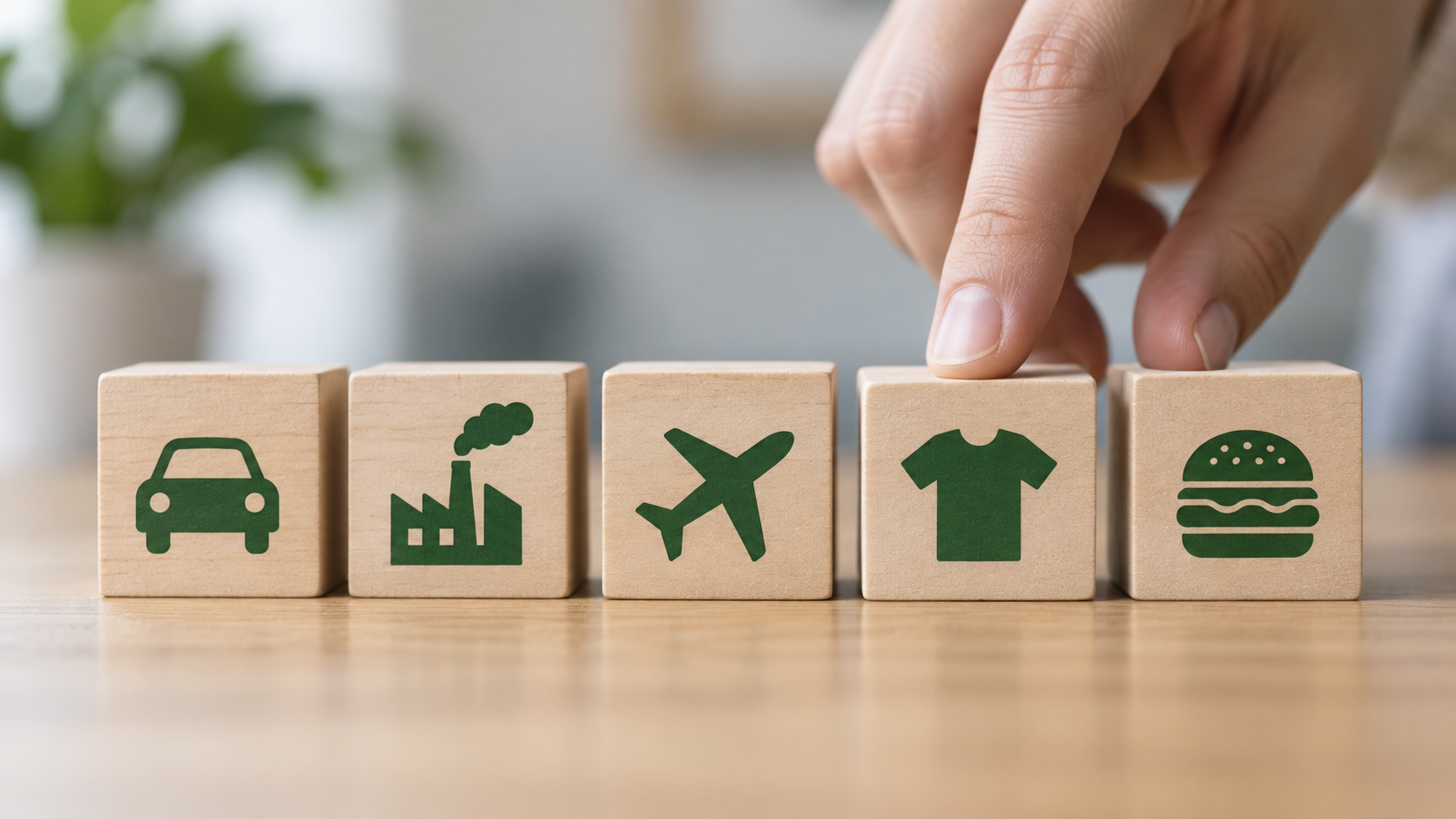
    Most of us know that a car exhaust emits carbon dioxide. But what about the steak on our plate, the electricity charging a phone, the shirt we are wearing, the sofa in the living room, or a two-hour flight? None arrives with a visible cloud of emissions attached to it. Yet each has a carbon history.

    That history is often hidden in another place or another time: at a power station, on a farm, in a mine, at a factory, aboard a cargo ship, or in the materials used to make a product. A personal carbon footprint is therefore not one activity. It is the combined result of everyday life moving through larger systems of energy, agriculture, manufacturing and transport.

    CO₂ means carbon dioxide. CO₂e, or carbon dioxide equivalent, is a wider measure that also expresses the warming effect of other greenhouse gases, including methane and nitrous oxide, in a common unit.

    A familiar journey by car

    A car journey is one of the few everyday activities where emissions feel tangible. For a representative average petrol car, travelling 100 kilometres is associated with roughly 16 kg CO₂e. In this simplified example, the vehicle’s manufacturing and road infrastructure are not included; a full lifecycle assessment would include both.

    What changes most immediately is not the road or the engine, but the number of people sharing the trip. The car travels almost the same journey whether one person is inside or three.

    People in the carApproximate emissions per person for 100 km
    1 personAbout 16 kg CO₂e
    2 peopleAbout 8 kg CO₂e
    3 peopleAbout 5–6 kg CO₂e

    These are representative figures based on the UK Government greenhouse gas reporting conversion factors. Exact results depend on vehicle size, fuel, engine efficiency, driving conditions and occupancy. The useful insight is simple: sharing a journey changes the emissions attributable to each traveller.

    Why flying is harder to estimate

    Flight time alone does not tell the whole story. Take-off, climb, cruise and descent use fuel differently, while aircraft type, passenger occupancy, cargo and the actual route all matter. The ICAO Carbon Emissions Calculator uses route-specific aircraft data, fuel consumption, passenger load factors and cabin configuration rather than a single universal number.

    As illustrative economy-class examples, a return journey of roughly 1,000 km may be associated with about 100–130 kg of direct CO₂ per passenger. A return journey of roughly 2,400 km may be around 200–250 kg CO₂ per passenger. These are not universal values, but useful scale markers for routes that might be scheduled around one and two hours each way, respectively.

    These figures describe direct CO₂ from aircraft fuel combustion. Aviation also has non-CO₂ climate effects at altitude. Those effects matter, but methods for estimating them differ, so it is more accurate not to apply one fixed multiplier casually. ICAO explains its approach in its calculator methodology.

    The carbon footprint on the plate

    Breakfast can look ordinary: coffee, milk, eggs, toast, perhaps fruit. Yet food is one of the clearest examples of why emissions cannot be understood only by looking at transport. What we eat often matters more than how far it travelled.

    The global averages below draw primarily on Poore and Nemecek’s 2018 research, published in Science and presented by Our World in Data. The underlying study covered about 38,700 commercially viable farms in 119 countries and 40 food products. Its lifecycle estimates include major parts of the supply chain: land-use change, farm emissions, animal methane, feed, fertilizer, processing, transport, packaging and retail.

    FoodApproximate global mean lifecycle emissions
    Beef from beef herds~60 kg CO₂e per kg
    Lamb and mutton~24 kg CO₂e per kg
    Cheese~21 kg CO₂e per kg
    Dark chocolate~19 kg CO₂e per kg
    Coffee~17 kg CO₂e per kg
    Farmed shrimp~12 kg CO₂e per kg
    Pork~7 kg CO₂e per kg
    Poultry~6 kg CO₂e per kg
    Farmed fish~5 kg CO₂e per kg
    Eggs~4.5 kg CO₂e per kg
    Rice~4 kg CO₂e per kg
    Milk~3 kg CO₂e per kg or litre
    Tofu~3 kg CO₂e per kg
    Tomatoes~1.4 kg CO₂e per kg
    Wheat and rye~1.4 kg CO₂e per kg
    Peas~0.9 kg CO₂e per kg
    Bananas~0.7 kg CO₂e per kg
    Apples~0.4 kg CO₂e per kg
    Root vegetables~0.4 kg CO₂e per kg

    They are global averages, not labels for every farm or every meal. Actual values can vary substantially between production systems and places. Still, the broad pattern helps explain why the invisible parts of food production—especially land use, livestock methane and farm inputs—can be so consequential.

    Why “processed” is not one category

    Processing can add energy use, ingredients, refrigeration and packaging, but it does not create one universal carbon value called “processed food.” The underlying ingredients still matter greatly. A lifecycle assessment of cooked ham reported about 13.4 kg CO₂e per kg, while noting earlier French estimates of about 7.7–8.6 kg CO₂e per kg. That range, documented in a 2021 lifecycle study of ham processes, is a reminder that product and production details matter.

    A processed vegetable product can look very different. One lifecycle study found about 0.72 kg CO₂e per kg for fresh-cut vegetables and 0.86 kg CO₂e per kg for pre-cooked vegetables. Processing is part of the story, not the whole story.

    The electricity behind the socket

    Plugging in a laptop or phone produces no visible exhaust. But the footprint of that electricity can differ enormously according to how it was generated. A useful comparison looks at lifecycle emissions, not only what leaves a smokestack. That means considering construction, materials, fuel extraction where relevant, operation, maintenance and eventual decommissioning.

    Electricity sourceLifecycle rangeApproximate emissions per 1 MWh
    Coal751–1,095 g CO₂e/kWh~750–1,100 kg CO₂e
    Natural gas combined cycle403–513 g CO₂e/kWh~400–510 kg CO₂e
    Nuclear5–7 g CO₂e/kWh~5–7 kg CO₂e
    Onshore wind8–16 g CO₂e/kWh~8–16 kg CO₂e
    Offshore wind12–23 g CO₂e/kWh~12–23 kg CO₂e
    Solar PV8–83 g CO₂e/kWh~8–83 kg CO₂e
    Hydropower6–147 g CO₂e/kWh~6–147 kg CO₂e

    These representative lifecycle ranges come from the UNECE Life Cycle Assessment of Electricity Generation Options. Technologies without combustion during operation are not literally zero-carbon: steel, concrete, silicon, copper, mining, construction and decommissioning all have emissions. Yet lifecycle studies show that their overall emissions can remain dramatically lower than fossil-fuel generation.

    The grid has a footprint too

    Generation is only part of the journey. Electricity reaches a wall socket through transmission lines, distribution networks, substations, transformers, cables, steel towers, copper, aluminium, concrete, maintenance and replacement infrastructure. Grid lifecycle footprints vary strongly between countries and system designs, so there is no responsible single number to add to every source of electricity.

    Grid losses also mean that slightly more electricity must be generated than ultimately reaches a home or business. A kilowatt-hour at the socket has a physical system behind it, even when that system is out of sight.

    The life before a garment

    A cotton T-shirt or pair of jeans can seem like a simple object. Before it is worn, however, cotton or synthetic fibres must be produced, spun, woven, dyed, sewn, packaged and transported. There is no responsible universal carbon value for “one shirt”: material, weight, factory energy, dyeing, production location and product lifetime all change the result.

    At a broader level, the European Environment Agency estimates that the supply chain associated with textile consumption by EU households produced roughly 355 kg CO₂e per person in 2022. This is embodied emissions: much of the climate impact was created before a garment reached a wardrobe.

    What a sofa carries

    Furniture becomes almost invisible once it settles into a home. A sofa or dining table looks passive, but much of its footprint was created before delivery: wood harvesting, metal production, foam, textiles, adhesives, manufacturing, packaging, transport and end-of-life treatment.

    Furniture varies too much for one universal figure. As one product example—not an industry average—a published Environmental Product Declaration for a particular three-seat sofa reported a lifecycle footprint of approximately 218 kg CO₂e. The point is not that every sofa has that footprint, but that familiar household objects can carry substantial embodied emissions. Lifecycle research comparing furniture products reaches the same broader conclusion: materials, design, manufacturing and use assumptions all matter.

    The things we buy

    Detergent, cosmetics, smartphones, computers, televisions, mattresses, kitchen appliances, toys and packaging all have their own histories. Much of a personal footprint occurs somewhere we never see: a mine, farm, factory, power station, warehouse, cargo ship or recycling facility.

    The lifecycle is easy to describe even when it is difficult to measure precisely: raw materials, manufacturing, packaging, transport, use and end of life. Some products use most of their energy while operating; for others, the largest share may be embedded in materials and manufacturing. Where comparable lifecycle figures are unavailable, it is better to acknowledge that uncertainty than to invent a neat number.

    Making the invisible visible

    Our carbon footprint is not one cloud following us around. It is distributed across thousands of places, machines and processes. Some emissions come directly from things we can see—a car exhaust or an aircraft engine. Others happened months earlier, thousands of kilometres away, while making something we use every day.

    Understanding that difference does not mean every decision has to become a climate calculation. It simply gives us a clearer picture of what our choices physically require. And once an invisible impact becomes visible, it becomes easier to understand.

    Sources and further reading

  • What Your Carbon Footprint Really Means

    What Your Carbon Footprint Really Means

    Your personal carbon footprint is an estimate of the greenhouse gas emissions connected to how you live, especially travel, home energy, food and everyday consumption. It matters because it turns climate impact into something more understandable, so you can see where your biggest sources of emissions are and decide what to reduce or take responsibility for.

    At ATLAS, that understanding is the starting point. If you want to see how a footprint estimate can connect to measurable forest growth and long-term carbon removal, explore how ATLAS works.

    Why this number matters

    A personal carbon footprint is a simple way to understand how everyday choices add up over time. It is not a score of personal worth, and it should not be used to create guilt. Instead, it can help you see where your biggest sources of impact are and where thoughtful changes may matter most.

    For many people, the largest contributors are not surprising: travel, home energy, food, and consumption. What is surprising is how useful it can be to look at those areas together. A footprint estimate turns a broad environmental concern into something more concrete, personal, and easier to act on.

    What a footprint includes

    Most personal carbon footprint tools look at the activities that shape daily life. While every calculator uses its own method, the goal is usually the same: to estimate the emissions connected to how we live.

    • Transport: driving, flights, and other regular travel
    • Home energy: heating, cooling, electricity, and fuel use
    • Food: dietary patterns and how food is produced
    • Consumption: clothing, goods, services, and waste

    No estimate is perfect, but a useful estimate can still guide better decisions. The point is not precision down to the last decimal. The point is clarity.

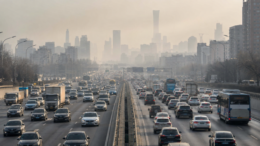
    multi lane highway with many cars and smog problem in the city

    How to use the result

    Once you know your footprint, the next step is to interpret it with care. A higher number does not mean failure, and a lower number does not mean the work is done. The value comes from identifying patterns and choosing realistic next steps.

    • Look for the categories with the biggest share of impact
    • Focus on changes you can sustain over time
    • Revisit your estimate as your habits change
    • Use the result as a starting point for learning, not an endpoint

    Good climate action starts with understanding, not perfection.

    Why Project Atlas exists

    Project Atlas was created to help people understand their personal carbon footprint and explore a more transparent, long-term approach to new forest creation. The aim is to make climate information easier to engage with while keeping the conversation grounded, responsible, and clear.

    That means avoiding exaggerated claims and focusing instead on understanding, transparency, and informed action. As the project develops, Insights will be a place for practical explanations, thoughtful context, and updates that help visitors navigate the topic with confidence.

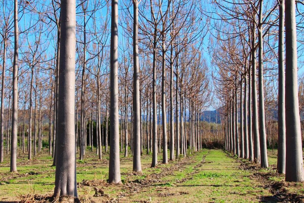
    Tree rows in a young forest landscape used as supporting concept imagery for Project Atlas

    A better place to begin

    If you are new to the idea of a personal carbon footprint, start with curiosity. Learn what shapes your impact, ask better questions, and look for actions that are meaningful in your own life. Small understanding can lead to better decisions, and better decisions can build momentum over time.

    That is the spirit behind Project Atlas: helping people move from uncertainty to understanding, and from understanding to responsible action. You can continue with more Insights or return to the ATLAS mission.